Case study: Overset Mesh Conservation for Isentropic Piston Compression in Star CCM+ - Femto Engineering - Femto Engineering

Case study: Overset Mesh Conservation for Isentropic Piston Compression in Star CCM+

In this article we are going to look at the conservation of several properties such as pressure, Temperature and density when modelling isentropic piston compression. We will model the motion of the compressing piston using an overset mesh method.

Introduction

An overset mesh is a type of mesh constructed from multiple overlapping grids. The primary advantages are the flexibility in handling complex geometries and the ability to handle relative motion between parts of the domain.

Interpolation takes place between the overlapping regions to ensure continuity. Interpolation can lead to numerical errors. Especially mass conservation can be an issue when working with overset meshes. This is because mass is not strictly conserved in overset mesh interfaces.

For single phase flows, Star CCM+ has the overset mesh conservation option. This option can be set to either: None, Flux corrections or Mass tracking. This case study aims to research the effectiveness of these mass conservation options. The subject of this study is a simple isentropic piston compression case. This case was selected, because the isentropic flow relations provide an exact solution. A comparison will be made between the results of the CFD simulations and the exact solution.

Geometry and mesh

The geometry and mesh of the piston are shown in Figure 1. A rectangular piston was chosen for this study. The grey surface at the bottom of the domain is the piston head, which moves up and down. The red outlined volume is the overset region.

The dimensions of the full piston volume domain are: 10 x 10 x 15 cm. The mesh of this domain is called the background mesh. For the background mesh 20 x 20 x 40 mesh cells are used. The dimensions of the overset region are 10 x 10 x 2 cm and consists of 20 x 20 x 16 mesh cells.


Figure 1   Piston geometry and mesh

Physics

As we have established in the introduction it is possible to obtain an exact solution for our problem using the isentropic flow relations. These relations are derived from the equation for entropy change. The entropy change for a calorically perfect gas, is given by:


When assuming reversible and adiabatic flow, the entropy change equals zero ( ).  The isentropic relations can then be derived from Equation 1:

In a closed system, conservation of mass applies. Therefore, the density is always equal to the mass divided by the volume.  This provides a relationship for pressure, temperature and density with respect to volume change.

For this case study a piston with a predefined motion is considered. Because the dimensions and motion of the piston are known, the volume over time can be calculated. This will then also provide the exact solution for density, temperature and gas.

The piston follows a sinusoidal motion. The vertical position (z) of the piston is given by:


Figure 2   Piston movement

The exact solutions for the density, pressure and temperature, which are obtained for this piston movement are shown in Figure 3. The compression ratio for this piston is 5:1.


Model setup

The physics models used in this simulation are:

  • Implicit unsteady
  • Inviscid flow
  • Segregated flow
  • Segregated temperature
  • Three-dimensional domain
  • Ideal gas law

The initial conditions and specific heat ratio used in the simulation are shown in Table 1.


Two parameters are varied between the different simulations. The first is the overset mesh conservation setting (None, Flux correction, Mass tracking).  Furthermore, the timestep is also varied (0.01s and 0.005s).

Results

The video below is provided to get an insight into the workings of the overset mesh.

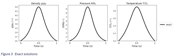
A comparison is made between the exact solution and the simulation results. The graphs below show the average density, pressure and temperature over the domain for the different overset mesh conservation setting. The exact solution is also plotted in the graphs.

The results shown in Figure 4 are from simulations with a relatively large timestep (dt = 0.01). Even though the mass tracking option yields better results in computing the compression rates, a slight lagging phase shift is present. When the timestep is halved (dt = 0.005), this phase shift decreases. This can be seen in Figure 5. The results for the other mesh conservation settings also improve, but not sufficiently.


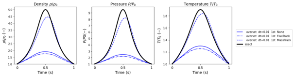
Figure 4   Results (with timestep: dt = 0.01)


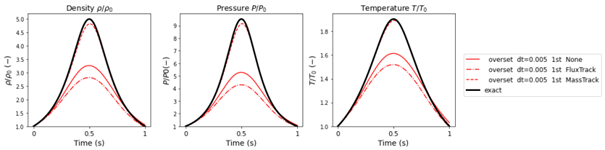
Figure 5   Results (with timestep: dt = 0.005)

The graphs clearly indicate that the results only come close to the exact solution when the mass tracking option is used. However, none of the overset conservation options provide a perfect solution. Interestingly, the flux tracking option does an even poorer job of conserving the mass during the simulation than having no overset conservation option at all.

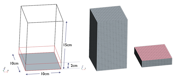
The reason for the poor performance of the flux correction has to do with the acceptor-to-active cells boundary. In an overset mesh the acceptor cell is a sort of “ghost cell” which receives information from all overlapping background mesh cells through the chosen interpolation scheme. The active cell then gets this information from the acceptor cell which is then used within the simulation.  The flux correction enforces the mass flux through the acceptor-to-active cells boundary to be zero and implements this in the pressure-correction equation. This boundary is defined by the overset interface in the region and the number of zero-gap layers. In this case, this boundary is located 2cm above the valve surface, as shown in Figure 6.


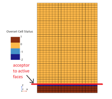
Figure 6   Acceptor-to-active cells boundary

Technically, a mass sink is located at this boundary in the domain 2cm away from the valve surface. In reality, mass should be able to move through these faces. A remedy could be to bring the overset interface closer to the valve surface. However, this also means that the background mesh needs to be refined to keep sufficient number of cells for the ZeroGap cell layer requirement. The density does return to  at the end of the simulation, which means that no mass is lost.

In contrary to the flux correction, mass tracking acts as a mass source rather than a sink. This source is added to the continuity equation. This is different than for the flux correction implementation where the pressure correction equation is modified. The mass tracking overset conservation corrects the mass at a certain point in time relative to the amount of mass that was initially present in the system. The difference in mass is added as a source term to the continuity equation.

Conclusion

In conclusion, when dealing with overset meshes in compressive cases, applying overset conservation is recommended to ensure accurate results. In STAR-CCM+, two overset conservation options are available: flux correction and mass tracking.

Flux correction acts as a sink in the pressure correction equation, preventing mass flux across the overset interface. This approach requires a very small overset region and a fine background mesh. Additionally, it performs poorly in simulations with high compression ratios, producing even worse results than using no overset conservation.

On the other hand, mass tracking introduces a source term to the continuity equation to correct for the mass deficit relative to the initial mass in the system. This method yields significantly better results in high compression cases, making it the preferred choice over both no overset conservation and flux correction. Mass tracking does necessitate the use of small timesteps due to a phase shift.

Overall, for compressive cases in CFD simulations using STAR-CCM+, mass tracking with a sufficiently small timestep is recommended for achieving the best results.

see the CFD tuesday video as an example here below:


September 16, 2024
get in touch

Do you need more information or want to discuss your project? Reach out to us anytime and we’ll happily answer your questions.

about us

At Femto Engineering we help companies achieve their innovation ambitions with engineering consultancy, software, and R&D.
We are Siemens DISW Expert Partner for Simcenter Femap, Simcenter 3D, Simcenter Amesim, Simcenter STAR-CCM+ and SDC verifier. Get in touch and let us make CAE work for you.

Privacy policy

×

Be ahead in FEA & CFD

Sign up for our newsletter to get free resources, news and updates monthly in your inbox. Share in our expertise!